A dynamical system can be used to model a particular physical phenomenon of interest. It is common to have systems affected by additive perturbations. Explicit performance bounds, for such systems, are desirable. The concept of input-to-state stability (ISS) may sometimes provide a conservative performance bound for systems subjected to bounded time-varying disturbances. Compared to results based on ISS, it may be possible to establish more aggressive bounds on system performance by finding invariant sets. The shape and size of such an invariant set will depend on the properties of a system. This work focuses on developing a computational algorithm for finding invariant sets for systems subjected to bounded additive disturbances. These sets are named robust forward invariant sets (RFIS) as per [1]. The authors in [1] provide analytical tools to construct robust forward invariant hexagons under bounded disturbances. Our goal is finding the smallest RFIS to obtain the tightest bounds on system performance. There exist many ways to construct invariant sets for dynamical systems. However, most methods existing in literature are analytical and valid for specific types of systems, or use numerical methods assuming some shape for an invariant set (enforced by the choice of a particular Lyapunov function). Minimizing the area occupied by sublevel sets of such a Lyapunov function, constrained by system dynamics, provides an estimate of a smallest invariant set. Since the shape is assumed apriori, it is not necessary that the solution obtained provides the smallest RFIS. Our work for computing an RFIS does not use Lyapunov functions or any particular optimization procedure. Newton-type methods for estimating a region of attraction are not used. Existing methods used to estimate the entire domain of attraction are not extended. A new approach is proposed to compute an RFIS for a perturbed system inspired by the notion of ‘Hamiltonians’. The idea [2] involves discretizing a domain of interest and starting with an initial guess of the boundary of the required invariant set. The proposed method iteratively evaluates points along proposed new sections of a possible boundary for the required set. During each evaluation, the angle between the vector field, and the tangent vector to a section of the possible boundary curve for the required set are compared. If the computed angle meets certain criteria, then the current point is stored as a possible choice for a boundary point. The choices for possible boundary points are updated every iteration. If the stored points satisfy certain termination criteria then the iterations stop and the required RFIS is found. Figures 1 and 2 show successful results obtained using the RFIS computation algorithm described here.
Figure 1. Results of using the RFIS computation algorithm on a version of the curve tracking problem
Figure 2. Results of using the RFIS computation algorithm with a simple system having circular trajectories
References
[1] M. Malisoff, F. Mazenc, and F. Zhang, “Stability and robustness analysis for curve tracking control using input-to-state stability,” IEEE Transactions on Automatic Control, vol. 57, no. 5, pp. 1320 – 1326, 2011.
[2] S. Mukhopadhyay, and F. Zhang “A path planning approach to compute the smallest robust forward invariant sets,” American Control Conference, pp. 1845 – 1850, 2014.
Learned Hallway Passing Behavior
The goal of learned hallway passing behavior is to provide insight into lifelong learning in human robot interaction. This passing behavior takes place between a robot and a human bystander when they approach ‘head-on’ in a hallway. Both robot and bystander must deflect in order to avoid contact. And while the direction that the robot uses to pass can be programmed, the preferred passing direction of a bystander is an unknown preference. One that can experience a slow change over time and is subject to noise. And with any robot designed for lifelong human robot interaction, there are certain parameters that must be met to make the continued interactions a success. The robot behavior must remain within predictable bounds. The robot must be able to identify and correct errors without a human expert inputting the data. And the robot must meet user’s expectations of interactive ability. The learned hallway passing behavior is bounded with detectable errors, so the last constraint, meeting bystanders expectations is important. Meeting the bystander’s expectations means that the bystander does not attempt to pass along the same wall as the robot. It also means that the robot’s behavior must be predictable to a human, or put another way, robust to noise. And finally this is the reason that current solutions, which involve the robot stopping when it sees a bystander in the hallway, are not adequate. Since those behaviors imply to the bystander that the robot can have more meaningful interactions with them. To learn the human’s unknown preference in a robust way so that the robot can remain moving during interaction, an avoidance direction algorithm was developed, based off of, but more robust than the weighted majority algorithm. Like the weighted majority algorithm this avoidance direction algorithm does have error that is bounded by the amount of noise present in the system. In addition the avoidance direction algorithm’s robustness, measured by how often it switches preference for turning direction, is determined by the frequency of noise. And is adaptable. The more frequently noise shows up in the system the more robust the system becomes in ignoring that noise. For the initial test of this algorithm a Matlab simulation was created. It showed that the error observed was within the theoretical error bound. It also showed that the algorithm could adapt to the level of noise in a system. With the robot being able to learn how much noise is expected and ignore all noise under that level. When the noise became greater than that level, representing a human preference changing, the simulation was once again able to adapt to the direction.
Learned UUV Diver Interaction
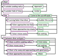
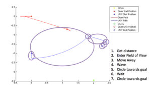
The goal of learned UUV (Unmanned Underwater Vehicle) Diver interaction was to create a learning algorithm that would find a safe, intuitive, and dynamical way of communicating its desires with a diver. In the set up of this problem safe means that the UUV never engages in behavior that would be risky for the diver such as getting too close, moving too fast or losing sight of the diver. In addition intuitive means that a diver could understand the commands without having to memorize the UUV vocabulary beforehand, and dynamical means that the only way that the UUV can communicate is by using motions. A two-dimensional simulation environment was created in MatLab. The simulated UUV had a set of ‘words’, basic moves which it could use to maneuver around the diver. In addition a basic diver dynamics were modeled, and the diver could either directly approach or move away from the UUV. The diver dynamics were based on a function of ‘Attention’, which was determined based of the UUV’s position in the divers cone of attention, personal space, the direction the UUV is facing, and the change in acceleration of the UUV. These parameters were chosen based on previous HRI research. From here a Temporal Difference Q-Learning algorithm was developed for the UUV to learn how to lead a diver towards a goal location. The states chosen were all considered to be relative to the diver, and included the separation between the diver and the UUV, the relative UUV orientation, and the UUV velocity. The actions that the UUV could perform at each step were a set of words that consisted of moving towards or away from the diver, circling the diver, waving or not moving. The reward was based off of the movement of the diver towards a goal point and not breaking any of the safety constraints. The program was run for 5,000,000 trials. And resulted in sets of words that were linked together to form ‘sentences’ that could be seen throughout various relative start positions of goal and UUV.
For several decades, autonomous underwater vehicles (AUVs), an instrument platform has been employed in oceanographic research. The small, mobile, and low-cost AUVs allow oceanographers to collect useful environmental data to characterize and model various oceanic environments such as open and coastal seas. However, ocean spatial and temporal variability significantly influence the paths of the vehicles because of their low velocities. Predicting the real trajectory of the vehicles becomes a challenging domain of research. To predict the route of the vehicles, many people have been using various ocean models that represent highly nonlinear time-varying dynamics of an ocean flow field. However, they have a variety of uncertainties: space and time sparseness of observational data sets and missing physics such as flow interaction. One approach to predicting the real trajectories of the vehicles with controlled velocity input in ocean flows is controlled Lagrangian particle tracking (CLPT) [1]. This concept includes the controlled input of the vehicles within the framework of Lagrangian particle tracking (LPT), an approach to finding the position of particles freely advected in ocean flows. To predict the error growth of the vehicles in a real flow field, the authors in [1] have defined CLPT error as position error between model-based simulated trajectory and real experimental trajectory of the vehicles. They performed an analysis of CLPT error based on probability theory, which assumes that the ocean field has spatial variability. In addition, they were able to predict the constant biased ocean flow field relatively accurately using linearized CLPT error dynamics [2]. Our works extend the previous results of [2], which assume that the ocean field has constant flow. We focus on predicting the real trajectory of the vehicles with waypoint controller, which guides a vehicle approach the waypoint by canceling out the normal component of a flow with respect to lines connected between the vehicle and the waypoint. To handle uncertain time-varying nonlinear systems that represent the vehicles on the uncertain oceanic environment, we use polar coordinate system and perturbed system theory. Unlike the previous research, our nominal and perturbed systems based on perturbed system theory are the key framework to have analytical solutions of the systems. In addition, range and angle channel of the systems provide us with physical insight of the real trajectory. To obtain the analytical solution of each channel, we develop three-step process to deal with two different perturbation terms. The first step is that we analytically solve the equation of angle channel by perturbation method when the perturbation term of the range channel equals zero. The second step has the same as the first step except that the perturbation term of the angel channel equals zero instead of the range channel. Final step is that we use superposition method to obtain the analytic solution of full perturbed systems from results of the first and second steps. Figure 1 and 2 show successful results obtained using analytical solutions in CLPT described here.
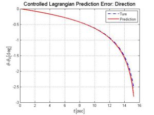
Figure 1. Comparison of true and analytical prediction error in angle channel
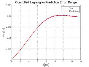
Figure 2. Comparison of true and analytical prediction error in range channel
References
[1] K. Szwaykowska and F. Zhang, “Trend and bounds for error growth in controlled lagrangian particle tracking,” IEEE Journal of Ocean Modelling, vol. 39, pp. 10–25, 2014.
[2] K. Szwaykowska and F. Zhang, “Controlled lagrangian particle tracking error under biased flow prediction,” in 2013 American Control Conference, Washington, DC, USA, 2013, pp. 92–98.
Curve Tracking Control for Autonomous Vehicles with Rigidly Mounted Range Sensors
Curve tracking control is fundamental for autonomous vehicles following desired paths, e.g. staying in lanes, or avoiding obstacles. An example in which this becomes relevant is when an autonomous vehicle is to follow the curb or the lane markings. Below figure shows the autonomous vehicle Sting-I that represented Georgia Tech in the DARPA Urban Grand Challenge in 2007. We designed a curve tracking control law in order to be used as a lane following component in the Georgia Tech Urban Grand Challenge system. It should be noted that our results may be applied to other types of autonomous vehicles with rigidly mounted range sensors. We briefly introduce our hybrid strategy of switching between control laws when the vehicle gets close to singularities. Define the safety zone such that once the vehicle enters the safety zone, then the vehicle will never leave and the curve tracking behavior is stabilized without collision. Now, the controller design problem is reconsidered so that the goal of the controller is to steer into the safety zone. Switching controllers, which steer the system into the safety zone in finite time, are depicted in the following figure. Rigorous proof and extensive simulation results verify the validity of the proposed switching control laws. 3D Simulations results are provided to demonstrate the effectiveness of switching control laws (see cylinder3.mpeg attached below). In the following figure, MATLAB simulation result is depicted. This figure shows a vehicle circling a lane-shaped curve in the clockwise direction starting from multiple initial positions. We vary the vehicle’s initial x-coordinate from -8 to 8, and y-coordinate from -6 to 6 with initial orientation 135 degree measured counterclockwise from the x-axis.
Battery Level Estimation of Mobile Agents Under Communication Constraints
Consider a team of mobile agents monitoring large areas, e.g. in the ocean or the atmosphere, with limited sensing resources. Only the leader transmits information to other agents, and the leader has a role to monitor battery levels of all other agents. Every now and then, the leader commands all other agents to move toward or away from the leader with speeds proportional to their battery levels. The leader then simultaneously estimates the battery levels of all other agents from measurements of the relative distances between the leader and other agents. We propose a nonlinear system model that integrates a particle motion model and a dynamic battery model that has demonstrated high accuracy in battery capacity prediction. The extended Kalman filter (EKF) is applied to this nonlinear model to estimate the battery level of each agent. We improve the EKF so that, in addition to gain optimization embedded in the EKF, the motions of agents are controlled to minimize estimation error. MATLAB simulation results are presented to demonstrate effectiveness of the proposed method. First figure shows the EKF by fixing the speed of an agent. Estimated battery level is shown in red, and true battery level is shown in blue. Initially, the difference between estimated battery level and true battery level is 1.5. However, after running the EKF within 17 time steps, estimated battery level converges to true battery level. Second figure shows the EKF by adjusting the speed of an agent periodically. At every 5 steps under the EKF, the speed of each agent is adjusted to minimize the error covariance predicted 5 steps forward in time. Initially, the difference between estimated battery level and true battery level is 1.5. However, after running the EKF within 6 time steps, estimated battery level converges to true battery level. Observe that, using adaptive speed gain, estimated battery level converges to true battery level faster than the case where fixed gain is used. In other words, time efficiency of the EKF increases using adaptive speed gain.
A provably complete exploration strategy by constructing Voronoi Diagrams
We address the problem of exploring an unknown workspace using a vehicle equipped with range sensors. Such sensors have the ability to determine a point on an obstacle boundary that is closest to the vehicle. We call such a point the closest point. If obstacle boundaries appear on both sides of the vehicle, then a closest point can be determined on each boundary. A path that is at an equal distance from these closest points is a Voronoi edge. All such Voronoi edges form the Voronoi diagram that reveals the topological structure of the workspace. If the vehicle visits all Voronoi edges in the workspace, then we consider the workspace as being completely explored. We present novel exploration algorithms, called Boundary Expansion algorithms, that enable the construction of Voronoi diagrams over unknown areas using a vehicle equipped with range sensors. The underlying control law uses range measurements to make the vehicle track Voronoi edges between two obstacles. This Voronoi edge tracking control law guarantees that the trajectory of the vehicle is smooth. The exploration algorithms make decisions at vertices in the Voronoi diagram to incrementally expand the already visited parts of the environment until a complete Voronoi diagram is constructed in finite time. Our exploration algorithms are provably complete, and the convergence of the control law is guaranteed. Simulations (see center_follow1.avi attached below) and experimental results (see success.avi attached below) are provided to demonstrate the effectiveness of both the control law and the exploration algorithms. The following figure shows successful experimental results of both the control law and the exploration algorithms. A robot is equipped with IR sensors to detect an obstacle environment. As the robot maneuvers in the workspace, a MATLAB plot is displayed in real time to show the detected obstacle environment. The real-time MATLAB plot is depicted above the corresponding obstacle environment. The robot is depicted as a dotted circle. In addition, the trajectory of the robot is plotted as a blue curve. On the trajectory of the robot, intersections are marked with small circles. In the MATLAB plot, a rounded rectangle is drawn around each intersection with a blocked sector.
Simultaneous Cooperative Exploration and NeTworking (SCENT) based on Voronoi diagrams in 2D environments
We develop strategies that enable multiple intelligent vehicles to cooperatively explore complex and dangerous territories. These strategies are called Simultaneous Cooperative Exploration and Networking (SCENT) algorithms. The workspace is considered completely explored if Voronoi diagrams are fully constructed. The vehicles are initially deployed at arbitrary locations and are not necessarily aware of the existence of other vehicles. Each vehicle starts with Boundary Expansion algorithms to explore its surroundings while deploying communication devices. Every vehicle drops communication devices and expands an information network while constructing a topological map based on the Voronoi diagram. As the information network weaved by each vehicle grows, intersections eventually happen so that the topological maps are shared. This allows for distributed vehicles to share information with other vehicles that have also dropped communication devices. A performance analysis of SCENT algorithms shows that in a bounded workspace, the time spent to complete the exploration decreases as the number of vehicles increases. We provide analytical formulas for this relationship. We verify the efficieny of SCENT algorithms through both MATLAB simulations (see center_follow2.avi attached below) and experiments using two mobile robots (see below for the link to SCENT experiments). First figure shows MATLAB simulations for one vehicle constructing Voronoi diagrams in a rectangular shaped workspace using Boundary Expansion algorithms. The inintial position of the vehicle is (2,20). The obstacle boundary is shown as red curve. The trajectory of a vehicle is plotted with blue points. Along the vehicle’s trajectory, the intersections are marked with large green dots. The exploration time is 99.05 time units. Second figure shows MATLAB simulations for two vehicles constructing Voronoi diagrams in a rectangular shaped workspace using SCENT algorithms. The initial positions of two vehicle are (2,20) and (45,2) respectively. The trajectories of two vehicles are marked with blue points and black circles respectively. The exploration time using two vehicles is 29.67 time unit which is less than one third of exploration time using one vehicle.
Capturing Multiple Intruders in a Graph Using the Information Network
As a result of SCENT algorithms, the information network is created concurrently with the topological map based on Voronoi diagrams in the workspace. The resulting information network and the topological map are used to solve complex and coordinated multi-robot tasks. We introduce an application of the constructed network to the problem of capturing multiple intruders in the workspace. We provide an algorithm to capture all intruders in an arbitrary connected graph. Based on this algorithm, we prove that the minimum number of searchers to capture all intruders in Voronoi diagrams (topological map of the workspace) is less than the number of obstacles in the workspace. Intruder capturing algorithm is implemented using an interactive simulation. In this simulation, an user generates an arbitrary connected graph and chooses initial positions of intruders in the graph. Then, using our algorithm, searchers are automatically deployed to capture all intruders.
Simultaneous Cooperative Exploration and NeTworking (SCENT) based on Voronoi diagrams in 2.5D environments
We extend SCENT algorithms from ground vehicles to aerial vehicles. In computer graphics and video game development, a 3D scene is often created using a 2.5D strategy in the sense that the movements of video game agents are confined within 2D planes. This strategy greatly reduces the possible outcomes associated with agent movements and the amount of computation needed to render real-time 3D visualization. As such, we introduce 2.5D SCENT algorithms so that multiple vehicles can explore 2.5D workspace in a time efficient way. A 2.5D workspace is composed of several 2D planes with different elevations. At each elevation, 2D SCENT algorithms can be applied, since 2D Voronoi diagrams are well defined. One major modification in 2.5D SCENT algorithms is that the information network has 3D structure, since a communication link exists between two nodes at different elevation. We further provide an analytical formula for the relationship between the number of vehicles and the time spent to complete the exploration and show that 2.5D SCENT algorithms lead to time efficient construction of Voronoi diagrams in an unknown 2.5D workspace. The following figure shows the illustration of 2.5D workspace. There are three sub-workspaces (2D planes) in this workspace. The rectangles with distinct color illustrate distinct obstacles in an 3D environment. Black dots in each sub-workspace illustrate positions of communication devices deployed at intersections on each plane.
Figure 1 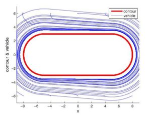
Figure 2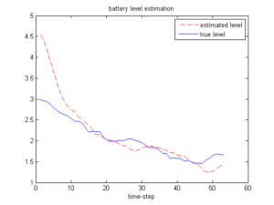
Figure 3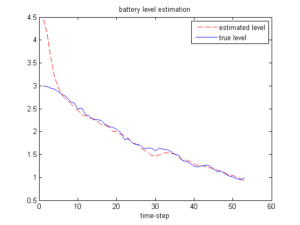
Figure 4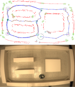
Figure 5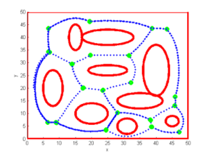
Figure 6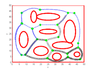
Figure 7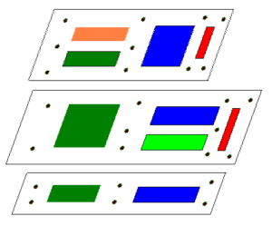 Figure 8
Cooperative Exploration of Level Surfaces in 3D Scalar Field
We develop strategies for a group of mobile sensing agents to cooperatively explore the level surfaces of an unknown 3D scalar field. To measure the field, a cooperative Kalman filter is constructed to combine the sensor readings from all agents and give the estimates of the field value and gradient. To reveal the structure of the field, the formation formed by the agents is controlled to track curves on a level surface in the field. We design steering control laws that are applied to the formation center to control the trajectory of the formation so that any curve with known curvature and torsion can be followed. In particular, we track lines of curvature on a desired level surface and the formation trajectory reflects the 3D geometry of the surface. The Taubin’s algorithm is applied so that a line of curvature can be detected and estimated. We prove the sufficient and necessary conditions that ensure the reliable estimates of the lines of curvature. We also investigate the problem of utilizing the minimum number of agents to accomplish the exploration tasks. Simulation results demonstrate that with the minimum number of agents, the lines of curvature on a desired level surface can be detected and traced successfully.
Robust Cooperative Exploration with a Switching Strategy
It has been observed that certain fish species switch between individual exploration behaviors and cooperative exploration behaviors based on different levels of food concentration in the ambient environment. Inspired by the biological observations, this paper develops a switching strategy for a group of robotic sensing agents to search for a local minimum of an unknown noisy scalar field. Starting with individual exploration, the agents switch to cooperative exploration only when they are not able to converge to a local minimum at a satisfying speed using the information collected individually. We derive a cooperative H infinity filter to provide estimates of the field value and the field gradient during cooperative exploration, and give sufficient conditions for the convergence and feasibility of the filter. The switched behavior from individual exploration to cooperative exploration results in faster convergence to the local minimum, which is rigorously justified by the Razumikhin theorem. We propose that the switching condition from cooperative exploration to individual exploration is triggered by a significantly improved signal-to-noise ratio (SNR) during cooperative exploration. The agents switch back to individual exploration when noises in the time-varying field has significantly reduced, which provides possibility for successful individual exploration. In addition to theoretical and simulation studies, we develop a multi-agent testbed and implement the switching strategy in a lab environment. We evaluate the exploration performance of a group of mobile robots sensing a light field under different sets of parameters. We have observed consistency between theoretical predictions and experimental results. In addition, the experiments demonstrate that the switching strategy is robust to perturbations resulting from unknown noises and communication delays.
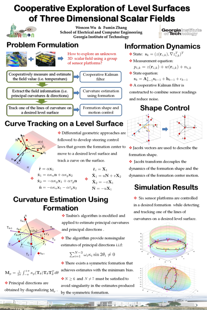
Figure 1
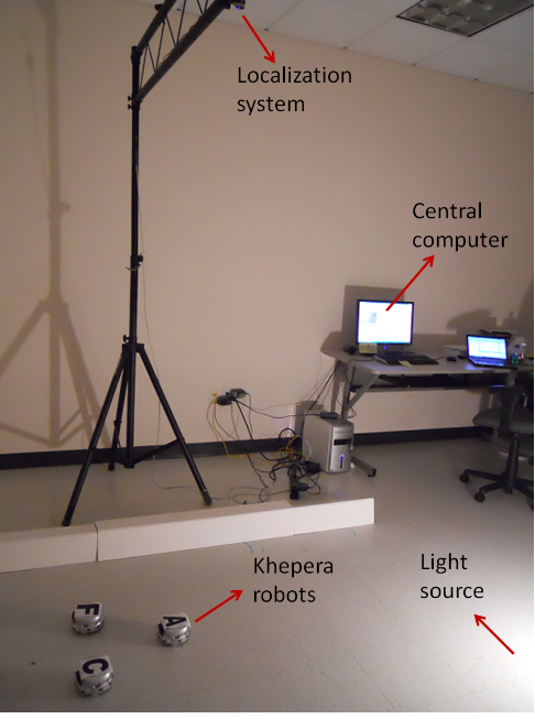
Figure 2. Experimental setting
Figure 3. Trajectories of the robots in the experiment (from individual exploration to cooperative exploration)
We developed middleware that that allows information to flow between sampling platforms deployed in the water to flow into simulations of the water’s dynamics, and to GCCS, the Glider Coordinated Control System, to provide navigation support for underwater vehicles. I am adapting GCCS to provide navigation support for the EcoMapper AUV. I’m very interrested in improving AUV guidance using the ROMS Ocean Model. My introduction to robotics consisted of working with Slocum Underwater gliders at the Rutgers University Coastal Ocean Observation Laboratory . This experience kindled my interest sampling the ocean, underactuated control in non-linear flows with large environmental uncertainty, building underwater robots and teaching. During my first year in Savannah, I lead GTSR (then GTS-AUV) to complete the ‘Alpha’ ROV, taught high school students participating in the Explorer post problem and served as head judge in the regional Lego robotics tournament. I am primarily focused on simultaneous localization and mapping of static and dynamic geophysical fields by submerged AUVs and AUV networks. At present, I am developing autonomous navigation algorithms for YSI’s EcoMapper vehicle. To enable the development and testing of autonomous navigation algorithms for the EcoMapper, and AUVs, ROVS and ASVs developed on campus, I am designing and deploying a facility for conducting aquatic robotics experiments on campus. To support the research group’s predictive sampling initiatives, I am developing simple in house implementations of the ROMS Ocean Model, which we will allow us to predict flow and assess environmental uncertainty. Access to water navigable by aquatic robots often limits the researchers’ opportunity to develop and validate underwater localization and mapping methods. Due to Georgia Tech. Savannah’s geographical location, our campus features on-site wetland area that we are developing for use by aquatic robots and networks. This testing area will consist of a dock, experimental water volume (up to 6m depth), a WI-FI network for surface communications and an acoustic global localization system. This resource will provide a safe, secluded environment that is under only natural forcing. During July 2010, a bathymetric survey of the lake was conducted, which covered most of our wetland. The resulting dataset was used to create a high resolution grid of the experimental area. We will, over time, complete and improve the accuracy of this map. We hope to expand our data coverage to include the missing region by exploring it with an Autonomous Vehicle. Last year, the LAMON research group obtained an EcoMapper AUV. We are currently developing methods for adjusting the vehicle’s underwater position estimate based on sonar measurements, a stochastic model of the measurement process and a prior knowledge consisting of bathymetric survey data. To support predictive sampling experiments both on site and in the open ocean, I am developing implantations the ROMS Ocean Model. The Regional Ocean Modeling System will allow us to predict the environmental flow based on satellite altimetry and in-situ observations. Flow estimates may be used for generating control input for autonomous vehicles such as predicting the source of a chemical contaminant given in situ measurements of the contaminant. I also support the LAMON by administering the LAMON server, website, blog, and provide webhosting support for GTSR and by helping to ‘make anything to work’.
We are addressing some of the problems associated with using acoustic communication to transmit control information to underwater vehicles. These problems stem from the time-delays present in acoustic communication links, which if not accounted for can significantly degrade the performance of underwater vehicle control, both when a vehicle is remotely-operated by a human or when multiple vehicles are collaboratively controlling each other. Furthermore, acoustic communication delays are difficult to model and predict, as they depend on a number of time-varying environmental factors and the motion of underwater vehicle. We have adopted a method to deal with these communication delays using passivity-based control that does not require a detailed model of the communication link.
Figure 1 illustrates the major features of our approach to using acoustic communication for underwater vehicle control. The critical part of this setup is the use of the scattering transform on both sides of the acoustic communication link to alleviate the problems with the communication delay. The scattering transform effectively smoothes out the signals being sent over the communication link, thereby preventing the delays from de-stabilizing the system. More precisely, the scattering transform is used to make the communication link passive. Passivity is a property of control systems that is very desirable in that connections between passive systems can be stabilized with negative feedback. What that means for this application is that as long as the other components, the human operator and the underwater vehicle controller, are passive then the overall system will converge, e.g. the underwater vehicle will accurately follow the control specified by the human operator.
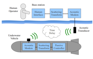
Figure 1. Passivity-based underwater vehicle control scheme
The strength of this approach is that it does not require that the length of the communication delays be predicted; the scattering transform handles any length of delay and the rest of the system can be designed as if there was no delay. This approach is also very flexible to alternate choices of input or controlled vehicles. While Figure x shows an example application of a human controlling a single vehicle, our approach could also be used for a human controlling multiple vehicles simultaneously or for multiple vehicles collaboratively controlling each other without human intervention. A couple of interesting applications of this are driving multiple vehicles in formation and using multiple vehicle to autonomously cover an area. Our contribution in this work include extending previous results in passivity-based trajectory tracking of robotic vehicles with delayed communications and applying these results to underwater vehicle control.
Controlled Lagrangian Particle Tracking
The goal of our research in Controlled Lagrangian Particle Tracking (CLPT) is the understand the motion of mobile robotic agents in complex ocean flow fields. Our focus is on using ocean models to inform navigation decisions for these autonomous agents, and using in-situ flow measurement data to update ocean model flow predictions. To compare the real-life performance of mobile underwater agents with simulations, we define the CLPT error as the difference in position between a mobile agent in the ocean, and a simulated agent moving in a flow field derived from an ocean flow model. The CLPT error limits the performance of ocean model-based control laws and can be implemented on the agent. Our investigation of the CLPT error is based on data collected in the 2006 Adaptive Sampling and Prediction (ASAP) experiment which was performed with underwater gliders in Monterey Bay, CA. The gliders were deployed to take measurements of ocean states along preset trajectories. A simultaneous virtual experiment was run, in which simulated gliders followed the same trajectories under a flow field derived from an ocean model (ROMS, NCOM, or HOPS). We observe that the CLPT error in this experiment exhibits similar growth for each ocean model used; the error increases exponentially until it reaches approximately twice the grid size used in the ocean model, and linearly thereafter. We have derived a lower bound on the steady-state CLPT error for an autonomous agent moving in a two-dimensional flow field. This lower bound is reached in finite time, and accounts for the change in the error growth rate. A dynamic programming approach has been implemented to generate optimal paths for an underwater glider to maintain minimal distance from a set goal point under the influence of flow. This approach uses a cost function that integrates the glider’s distance from the goal over a finite time horizon. The domain of operation is discretized in both space and time, and the cost-to-go and associated optimal control action are computed at each point in the discretized domain, starting at the final time (see Figure 2). The glider’s position is then integrated forward using a simple particle model for the glider dynamics. At each time step in the integration, the glider’s control action (e.g. the choice of heading angle) is taken to be a bilinear interpolation of the optimal control actions at the nearest states in the discretized domain. The glider’s total velocity is taken as a sum of the glider’s through-water velocity and the predicted flow velocity, which is obtained from an ocean model. This gives a near-optimal trajectory that can be converted to a waypoint list to be passed to the glider. The dynamic programming path-planning algorithm has been tested in the simulation module of GCCS, which uses ocean-model flow data and an approximated model of glider dynamics, as well as an implementation of the glider’s on-board control algorithms, to simulate glider motion given waypoint lists passed to the glider. We use controlled Lagrangian particle tracking to evaluate the accuracy of the simulated glider position. Errors in glider position simulation are due to limited resolution of ocean models, missing physics in the models, and sparseness of available ocean measurements used to drive the model. Using a modified Langevin equation to model the growth of the expected glider position error (termed CLPT error), we have shown that the magnitude of the expected error in simulated position grows exponentially until reaching a lower bound equal to twice the gridsize of the ocean model used (see Figure 4). The error growth then slows to a polynomial function of time.
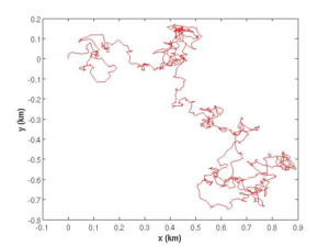 Figure 1. Sample trajectory of a particle moving with Langevin dynamics.
 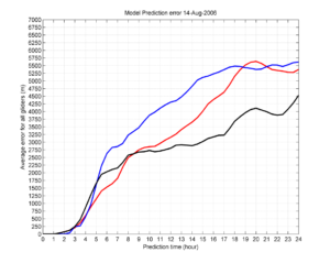 Figure 2. CLPT error growth over time in the ASAP experiment for different ocean models (ROMS, NCOM, and HOPS).
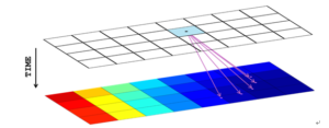
Figure 3. An illustration of dynamic programming for glider path planning. 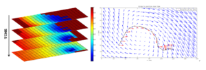 Figure 4. Dynamic programming-based path planning over a sample domain with a static flow field.
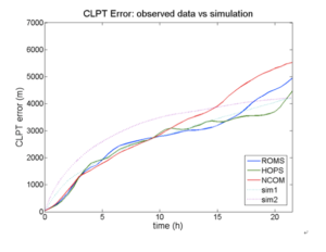
Figure 5. CLPT error growth over time. This data was collected during the 2006 ASAP experiment in Monterey Bay, CA.
Diagnosis and Prognosis of Scrubber Faults for Underwater Rebreathers based on Stochastic Event Models
Imperfect CO2 removal mechanisms of CO2 scrubbers often lead to the existence of CO2 in gas inhaled by a diver from underwater rebreathers. This may cause CO2 related rebreather faults and subsequently would increase the risk of human injuries. We introduce a stochastic model for three CO2 related rebreather faults: CO2 bypass, scrubber exhaustion, and scrubber breakthrough. We establish the concept of CO2 channeling that describes the cause of the faults and present a CO2 channeling model based on a stochastic process driven by a Poisson counter. This helps us to investigate how CO2 flow inside the rebreather is affected by CO2 related faults. Fault diagnosis/prognosis algorithms are developed based on the stochastic model and are tested in simulation.
Recent Status of the GCCS implementation for the Long Bay Project
1. Direct interface between the GCCS and the dock server. A direct interface between the GCCS and the dock server has been added to the GCCS. When a glider is in operation, glider terminal, which is an application provided by Webb to help glider users interact with gliders, keeps a record of all text output on the screen in a log file. The GCCS now directly accesses the dock server to e xtract necessary information such as surfacing position and time, and flow velocity to generate optimal waypoints from log files on the dock server without assistance of third party software. All the files of the collected data by a glider during the dive also contain necessary glider surfacing information for the GCCS to generate a list of waypoints, but it takes time to transmit the data files to the dock server via Iridium. In the new interface in the GCCS, this necessary information is taken from glider terminal log files as soon as it appears on the screen of the glider terminal, so the GCCS can generate a set of optimal waypoints while the collected data files are being transmitted from gliders to the dock server and can send this waypoints list as soon as the glider is ready after the file transmission .
2 . Incorporation of HYCOM in the GCCS. To analyze the behavior of the glider in the Long Bay, we first developed a simple tidal and Gulf Stream current model based on M2 tide and sinusoidal meandering motion of Gulf Stream, and then simulated gliders under the simple current model using the GCCS. Later, t o obtain more realistic simulation results, HYCOM (HYbrid Coordinate Ocean Model, http://www.hycom.org ) was used for glider simulations. In the Long Bay project, the GCCS generates a set of waypoints for a glider over the time horizon of at least 12 hours. In addition to the fact that Gulf Stream meanders and has unpredictable eddies, the ocean flow by Gulf Stream is often too strong for gliders to navigate through to get to the target. To deal with this the GCCS takes into account current or predicted flow velocities over the time horizon to generate optimal path. However, ocean model forecast files contain forecast data over the limited forecast time period, so for multiple days of implementation the GCCS needs to switch between ocean model forecast files corresponding to the date, the flow prediction data of which the GCCS needs. T he GCCS is now able to run for a multiple day experiment, which needs one or more sequential ocean model forecast data files.
3. Simple glider navigation algorithm for virtual mooring (Station keeping). In the Long Bay experiment, one glider will be trying to maintain its fixed surfacing position , being operated as a quasi-fixed position profiler . In the GCCS, glider s are modeled as particles traveling at constant speed relative to flow. Since the flow is not constant in general, the relative glider speed is not constant due to the influence of flow. If we want a glider to reach a given position, we need a navigation algorithm to create a list of w aypoints for the glider between its current position and the desired position. A simple glider navigation controller is designed to perform this behavior. Figure 1 shows the domain of the Long Bay with two gliders. The one at (-78.1°, 32.95°) near the red dot will perform virtual mooring.
4 . Planned future events. (a) Using HYCOM ocean model forecast data, a hindcast simulation is planned for the time period over which a real glider was deployed by UNC in the Georgia Bight in August 2006, trying to hold station at 30.8 ° N, 81.316 ° W. (b) SABGOM ocean model forecast data, which would have more frequent forecast intervals than HYCOM, will be also provided for a better emulation of the flow field.
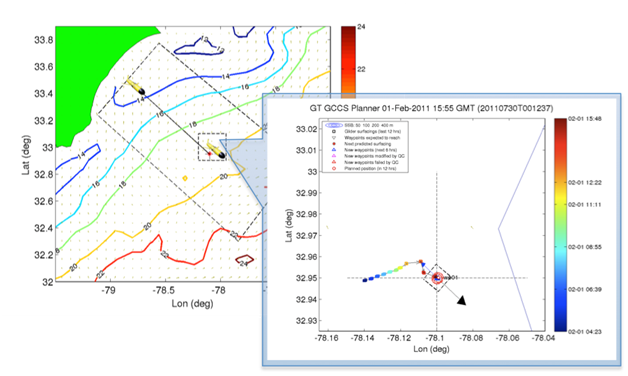
Figure 1 . In (a), outer dotted box represents t he domain of the Long Bay project, inner dotted box is used for the m ain focus region for a virtual mooring glider . The colored contours represent SST field in the domain, and the arrows, which cover the entire field, show the flow field in the domain. In (b), it shows the implementation of the simple glider navigation algorithm for the virtual mooring glider in the GCCS. Colored rectangles represent glider surfacing positions with corresponding time in the color bar.
We have operated the Ecomapper in two modes. The Ecomapper can be drove manually when it is on surface and within Wi-fi range. In this mode, information about the EcoMapper is displayed on the Underwater Vehicle Console (UVC) but are not recorded by the EcoMapper. The information displayed include the speed, position (Latitude and Logitude), and heading, as well as sensory data that includes temperature, salinity, depth and altitude. • Autonomous mode. In this mode, the Ecomapper follows a predefined course, either on surface or below surface, independently of the user. During missions, the Ecomapper records all sensor measurements into log files. W e can get the following data from the log files after the Ecomapper finishes a mission: Ecomapper positions (latitude and longitude), velocity, pitch angle, roll angle, depth from surface, height to bottom, temperature, sound speed, salinity.
What we have achieved with the Ecomapper
We successfully surveyed the west pond in Georgia Tech Savannah Campus (see Figure 1) autonomously using the Ecomapper. Autonomous missions both on surface and below surface were executed successfully. Bathymetry data were collected during the missions. Figure 2 shows the courses the Ecomapper followed and the bathemetry data collected. By interpolating the raw depth data, we built a bathemetry map for this pond (see Figure 3). The averaged salinity in this pond is around 0.09 ppt (parts per thousand).
As part of the project “Collaborative Research: RAPID: Autonomous Control and Sensing Algorithms for Surveying the Impacts of Oil Spills on Coastal Environments” supported by NSF, the EcoMapper was deployed to survey the retention pond located at the Grand Isle State Park (see Figure 4) in Louisiana . Five autonomous missions between surface and 0.5 meters below surface were executed. We did not let the Ecomapper dive deeper since the pond is shallow, with maximum depth 1.65 meters. The data collected show that the temperature and salinity does not change much with depth (salinity changes<0.5ppt, Temperature changes<1 o C) as the lagoon is shallow. Figure 5 shows the courses the Ecomapper executed and the bathemetry data collected. By interpolating the original depth data, we obtained a bathemetry map for this pond (see Figure 6). The salinity of the lagoon varies between 13ppt and 17 ppt under different weather condition.
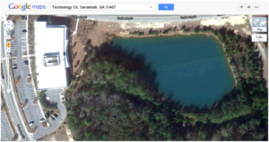
Figure 1. 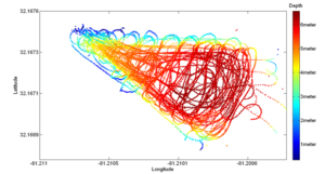
Figure 2. 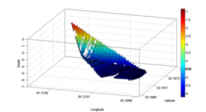
Figure 3.
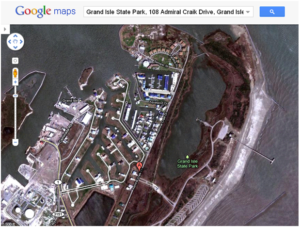
Figure 4. 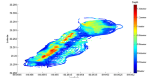
Figure 5. 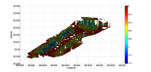
Figure 6.
